Before analysis, researchers should consider conducting finer-scale
filtering in order to clean the NestWatch dataset after running nw.cleandata().
This may include selecting certain species, identifying specific nest
phenology dates (i.e., incubation should not last longer than X days for
species Y), or limiting nest attempts to a certain geographic area.
Filtering Species
Limiting the dataset to just a few species can easily be done using
the pipe (%>%). If you are unfamiliar with “piping”, see
the migritrr
package. Below we will subset the version 1 of the NestWatch dataset to
include only attempts for Bewick’s Wren (“bewwre”) and Carolina Wren
(“carwre”). The code below walks through download, merging, and
filtering to species from scratch.
Note that subspecies and identifiable forms of species have different
species codes than the main species. For example, Carolina Wren’s
species code is “carwre” but Carolina Wren (Northern) has the code
“carwre1”. If you wish to include all subspecies/forms, make sure to run
nw.cleantaxa(data = data, rollsubspecies = T) or lookup the
species codes you would like to include by referencing the eBird
taxonomy table using auk::ebird_taxonomy.
library(nestwatchR)
library(dplyr)

# Download and merge datasets
nw.getdata(version = 1)
nw.mergedata(attempts = NW.attempts, checks = NW.checks, output = "merged.data")

# Filter data to include only carwre and bewwre
wrens <- merged.data %>% filter(Species.Code %in% c("carwre", "bewwre"))

# View what species are in the new dataset
unique(wrens$Species.Name)
> [1] "Carolina Wren" "Bewick's Wren"
This “wrens” data subset from dataset Version 1 is also included
within the package for quick access using
wrens <- nestwatchR::wren_quickstart:
Filter Spatially
Spatial filters are a flexible way to limit data to a predefined
geographic area. You may choose to limit an analysis to nesting attempts
within a certain area, like a single Bird
Conservation Region or a select political jurisdiction. Or you may
choose to remove potentially misidentified species by using a range map
to filter out nesting attempts. If those filtering criteria are easily
subset from the dataset, like states/provinces and countries (via
Subnational.Code), you can quickly use subsetting rules to
filter the data for analysis. But, if those criteria are not already
easily subset-able, a spatial filter can be a good option.
As an example, we can first view a plot of where the nests in
wrens are located by species. Here we will use the package
tmap
to produce an interactive map. We will also be utilizing the sf package to
help create and transform our tabular data into spatial data. We will
then project the wrens data into the Lambert Conformal Conic Projection,
which is well suited for mapping areas in the United States (but you can
change the object proj to any appropriate PROJ.4 string for
the area you are mapping).
[!Note] If you are unfamiliar with working with spatial data, this is a good resource on coordinate reference systems and projections within R.
First, to limit stress on our plotting instrument, we will limit the dataset to include only one line of data for each nest. If you would like certain variables of the nest, like clutch size, fledge/fail date, or substrate, to be visible when you click on individual points, but sure to select those columns here. In this example, we will select clutch size and outcome.
# Select a few columns that your are interest in plotting
wrens <- wrens %>% select(Attempt.ID, Latitude, Longitude, Species.Name,
                          Species.Code, Clutch.Size, Outcome) %>%    # select columns
                   distinct()                                        # get one row for each nest
Now that we have a single line of data for each nest, we can plot our points. Do note that depending on your sample size, your map may take a while to plot. If you think this might be happening, try plotting just a subset of the points at a time or switching the tmap mode to “plot” (see tmap documentation for more details).
# Create a spatial object from nest data
library(sf)
nest_points <- sf::st_as_sf(wrens, coords = c("Longitude", "Latitude"), crs = 4326)  # data are in WGS 84 (crs = 4326)

# Define desired CRS for data projection
proj <- "+proj=lcc +lon_0=-90 +lat_1=33 +lat_2=45"  # PROJ.4 string defining the projection

# Project the nest points into LCC projection
nest_points <- sf::st_transform(nest_points, crs = proj)   # apply projection

# Map nest locations
library(tmap)
tmap_mode("view")                                       # starts interactive plot
map <- tm_basemap("Esri.WorldGrayCanvas") +             # define basemap
  tm_shape(nest_points) +                               # add nest point data
  tm_symbols(shape = 21,                                # defines shape as circle w/ border
             fill = "Species.Name",                     # define what colors map to
             fill.scale =                               # colors
                tm_scale_categorical(values = c("#457999", "#8DCA8B")),
             size = 0.5)
# View the map
map 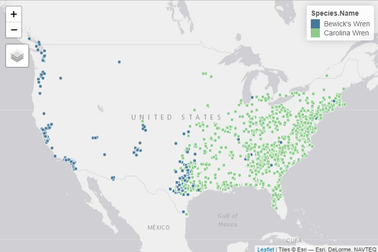
By looking at this map, we can see that there are several suspicious nests identified as Bewick’s Wrens in the eastern United States. Bewick’s Wrens are not typically recorded east of the Mississippi River, so some of these records could be misidentified. We could decide on a subset of states/provinces to filter out-of-range nest attempts, but a better method might be to filter nest locations based on a range map.
eBird Range Map Polygons
The eBird
Status and Trends Products contain a wealth of information on bird
populations. Among the available products are range maps of species for
which Status and Trend Models have been run. These data are easily
accessible in R through the ebirdst
package. To access these eBird data, you will need to acquire a free
access key. This key will give you access to Status and Trends Data
within R. For more information and to acquire an access key, see the documentation here.
We can use our unique access key to download the range map of
Bewick’s Wren and Carolina Wren. Note, you will need the 6-letter
species codes of those species you would like to download, not their
alpha code or common name. By modifying the access key, species, and
download location in the code below, you can download and open the range
polygons to your global environment. This code selects only the breeding
range layer if available, and if unavailable then selects the resident
range layer. Note: You only need to input your access key once (R will
store it for you!) and you only need to download the range maps once
(you may get an error if you rerun ebirdst_download_status()
when the data already exists at the spatialdata_path
location). You may also need to modify the year in the code below
depending on what Status & Trends data product is available.
# Obtain and set an ebird access key
library(ebirdst)
set_ebirdst_access_key("pasteyourkeyhere")      # you only need to do this once, R will remember it

# Define what species you want to download by their 6-letter code
spp <- c("bewwre", "carwre")

# Specify where the data will be downloaded
# Here we will reference a folder called "spatial" in our working directory:
spatialdata_path <- c("spatial")

# Download range maps by species
for (i in spp) {
  ebirdst_download_status(species = i, download_abundance = FALSE,
                          download_ranges = TRUE, pattern = "_smooth_27km_",
                          path = spatialdata_path)
}

# You may need to modify the year below to reflect the appropriate S&T product that downloaded
# Read in the range files
for (i in spp) {
  # Generate the path to the .gpkg files
  file_path <- paste0(spatialdata_path, "/2023/", i, "/ranges/", i, "_range_smooth_27km_2023.gpkg")
  # Read in the .gpkg file
  range_data <- st_read(file_path)
  # Generate the name for the object
  object_name <- paste0(i, "_range")
  # Assign the value to the dynamically-generated object name
  assign(object_name, range_data)
  rm(range_data)
}

# Select just breeding layer if available, else resident layer
object_names <- paste(spp, "range", sep = "_")
for (i in object_names) {
  if (i %in% ls(envir = .GlobalEnv)) {
    data <- get(i, envir = .GlobalEnv)
    if (any(data$season %in% "breeding")) {
      data <- data %>% filter(season == "breeding")
      data <- data %>% st_transform(nest_points, crs = proj)
      assign(paste0(i), data, envir = .GlobalEnv)
    } else {
      data <- data %>% filter(season == "resident")
      data <- data %>% st_transform(nest_points, crs = proj)
      assign(paste0(i), data, envir = .GlobalEnv)}
    rm(data)
  }
}

# Clean up intermediate objects
rm(file_path, i, object_name, object_names, spatialdata_path)
Now that we have range polygons for Bewick’s Wrens and Carolina
Wrens, we can add them to our map and investigate our nest locations a
bit closer. Let’s plot just the Bewick’s Wren data.
# Subset nest locations to Bewick's Wrens
bewwre <- nest_points %>% filter(Species.Code == "bewwre")

# Map the nests onto the range polygon
tmap_mode("view")                                     # starts interactive plot
map <- tm_basemap("Esri.WorldGrayCanvas") +           # define basemap
  tm_shape(bewwre_range, name = "Bewick's Wren") +    # add range polygon
    tm_polygons(fill_alpha = 0.5,                     # polygon transparency
                fill = "#B4CFE1",                     # polygon fill color
                col = NULL) +                         # polygon border color
  tm_shape(bewwre) +                                  # add nest points
  tm_dots(fill = "Species.Name",                      # define how to color points
          fill.scale =                                # define point fill
            tm_scale_categorical(values = c("#457999")))
map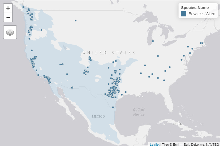
We can now see that there are more than a few nests outside of the
typical Bewick’s Wren range. But a few of these nests are also close to
the range border and may truly belong to Bewick’s Wrens. We can
use nw.filterspatial()
to help us identify and/or remove nest attempts outside of the range
polygon (or any other shapefile you may want to filter by).
nw.filterspatial()
requires the input of sf objects for points =
and polygon =, representing the nest points to be filtered
and the shapefile by which they are filtered, respectively. The
mode = argument is used to define if points identified
outside the polygon should be flagged for review (“flagged”) or removed
from the dataset (“remove”). This function also has an optional buffer
argument buffer = where the user may define a distance
outside the polygon for which nest locations will be allowed. This
distance can be either in kilometers or miles and should be defined
using buffer_units = "km" or = "mi". The
resulting buffer polygon may be optionally exported to the global
environment for saving or plotting using the logical
buffer_output = T. The user may also define their desired
projection using proj = and inputting a PROJ.4 string. If a
projection is not provided, then the function will default to the
Lambert Conformal Conic which is well suited for plotting the majority
of NestWatch data at this time. Finally, the optional
output = argument can be used to name the resulting
spatially-cleaned dataframe.
If we zoom in to central Colorado, we can see there are a few Bewick’s Wren nests just outside the range border.
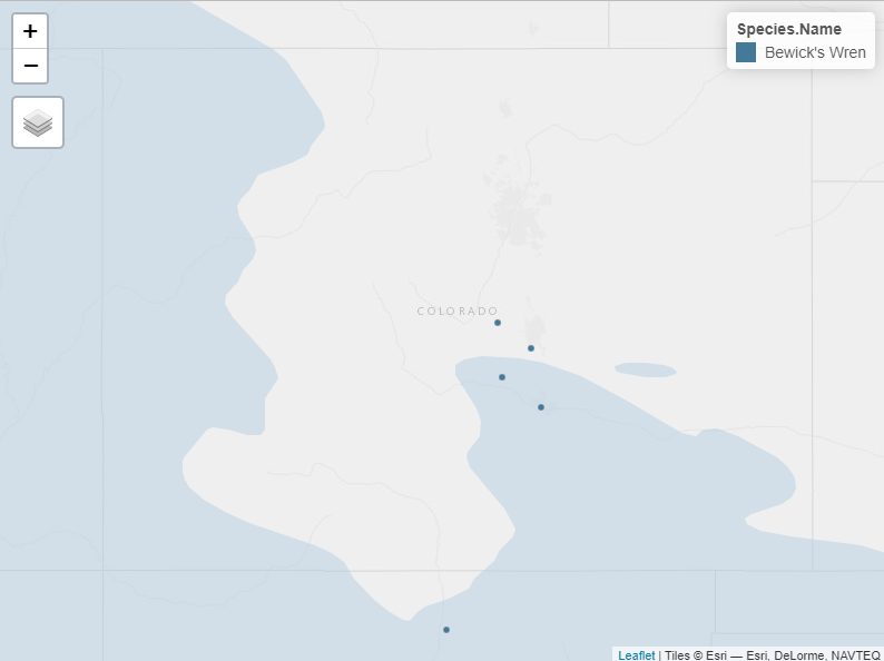
We might choose to keep nests like these in our analysis, because they could be correctly identified and just a bit outside the typical range. Let’s define a buffer zone to keep such nests but exclude those well outside the expected range:
nw.filterspatial(points = bewwre,                    # Bewick's Wren nest points
                 polygon = bewwre_range,             # Bewick's Wren range shapefile
                 mode = "flag",                      # flag points outside
                 buffer = 50,                        # add a 50km buffer zone
                 buffer_units = "km",                # units = km
                 buffer_output = T,                  # yes, output the buffer polygon
                 proj = "+proj=lcc +lon_0=-90 +lat_1=33 +lat_2=45",   # LCC from above
                 output = "flagged_nests")           # define the output name
We can plot the results to see which points were flagged for
review (and would be removed if mode was set to “remove”):
# Relabel nests within range for nice map symbology
flagged_nests$Flagged.Location[is.na(flagged_nests$Flagged.Location)] <- "In-Range"

map <- tm_basemap("Esri.WorldGrayCanvas") +                 # define basemap
  tm_shape(shp = polygon_buffered, name = "50km Buffer") +  # add buffered polygon, define color
  tm_polygons(fill_alpha = 0.5, fill = "#CEE6F3", col = NULL) +
  tm_shape(shp = bewwre_range, name = "Bewick's Wren Range") +  # add range polygon, define color
  tm_polygons(fill_alpha = 0.5, fill = "#B4CFE1", col = NULL) +
  tm_shape(flagged_nests) +                                 # add nest points, color by "Flagged.Attempt"
  tm_dots(col = "Flagged.Location",
          palette = c("#B31B1B", "#457999"))
map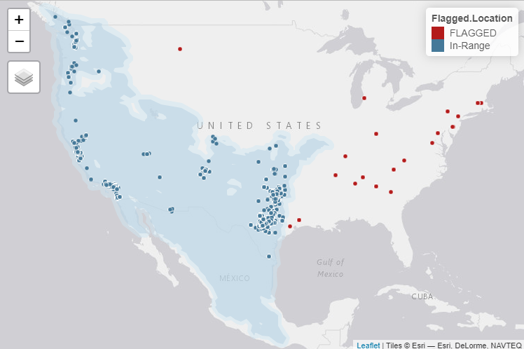
We can now quickly filter out those nests with flagged locations outside of our defined range.
# Remove flagged attempts
nests_cleanlocs <- flagged_nests %>% filter(Flagged.Location == "In-Range")
Filter Using Nest Phenology
You may also choose to refine the coarse phenologic filtering done in
the cleaning process of nw.cleandata().
NestWatch data are known to have some errors where participants either
enter dates incorrectly (i.e., enter the year portion of a date as 2021
in one field and 2020 in the next) or incorrectly continue a nest
attempt when it should be considered a new nest (i.e. nest usurpation or
failure-and-rebuild). As an example of the latter, if a bluebird nest
fails due to predation and the pair renests in the same box, this should
be entered as two different attempts at the same location. But records
of these “run-on nests” where the first attempt was not ended do exist
in the dataset. One way a user might choose to identify or remove such
nesting attempts, or ones which are outside of the expected nesting
timeline for a given species, is to use phenologic filtering.
Phenologic filtering allows the user to define the allowed maximum
number of days for each different period in the nesting cycle, or for
the whole nesting cycle. The function nw.filterphenology()
uses both the data in the attempt summary info (data originating from
the “Attempts” dataset) and the individual visits data (originating from
the “Checks” dataset). Note that NestWatch participants do not always
provide the summary info, but the key dates may be inferred from the
series of nest check data. Because the function uses both summary and
checks data, we highly recommend running the series of estimation
functions provided in the package to estimate summary dates where they
were not specifically provided by the participant (see: nw.estclutchsize(),
nw.estfirstlay(),
nw.esthatch(),
and nw.estfledge()).
Running these estimations can increase the amount of information
available for phenologic filtering.
For this function, a small user-created dataframe in the following format is needed. These values represent the maximum allowable number of days a nest of a particular species can be in each nesting stage. “Total” refers to the maximum number of days from the initiation of nest building though fledging. In this example we will continue using NestWatch data for Bewick’s Wren and Carolina Wren:
First, we will load, clean, and estimate missing values:
## 1. Load, Clean, & Estimate Data

# Load the supplied `wrens` dataset
data <- nestwatchR::wren_quickstart
length(unique(data$Attempt.ID))
#> [1] 7626
# > [1] 7626      # number of nesting attempts for Bewick's and Carolina Wren

# Run cleaning function
nw.cleandata(data = data,
             mode = "remove",
             methods = c("a", "b", "c", "d", "e", "f", "g", "h", "i", "j", "k"),
             output = "data")

# First, run summary date estimation functions:
# Missing summary data will be estimated, when possible, by using AVERAGE values
# for the focal species. The dataframe below contains values of the average clutch
# size, number of eggs laid per day, incubation period (in days), and nestling
# period (in days) which the estimation functions will use to estimate any missing values.
avg_phen <- data.frame(Species = c("bewwre", "carwre"),
                       Clutch.Size  = c(5, 4),
                       Eggs.per.Day = c(1, 1),
                       Incubation   = c(16, 16),
                       Nestling     = c(16, 13))

nw.estclutchsize(data = data, output = "data")
nw.estfirstlay(data = data, phenology = avg_phen, output = "data")
nw.esthatch(data = data, phenology = avg_phen, output = "data")
nw.estfledge(data = data, phenology = avg_phen, output = "data")
Now we can create the maximum allowable periods dataframe and
run phenological filtering. Here we choose the maximum values for
incubation, nestling, and total to be the mean value plus several days
to account for allowable variation in length. Again,
total = represents the maximum nesting period, spanning
between first build and fledge. For example here, Bewick’s Wren
typically build nests within 8 days. So we might say max build time is
10 days, and lay + incubation + nestling + build = 60 days:
## 2. Phenologically filter data by limiting dataset to nests with dates within the maximum possible range.

# Create simple df with maximum allowable # days in each nest phase for Bewick's and Carolina Wrens.
# You can provide data for a single species or multiple species to be run at the same time.
# We suggest adding a few days of buffer to average incubation, nesting, and total
# nesting period lengths. This is your judgement call based on the biology of the focal species.
max_days <-
  data.frame(species =  c("bewwre", "carwre"),
             lay = c(8, 6),           # max recorded clutch size for focal species
             incubation = c(20, 20),  # means plus a bit of buffer
             nestling = c(20, 20),    # means plus a bit of buffer
             total = c(60, 55))       # mean days build to fledge, plus a bit of buffer

# Filter attempts based on nesting phenology
nw.filterphenology(data = data,
                   mode = "flag",
                   max_phenology = max_days,
                   trim_to_active = TRUE,
                   output = "flagged_phenology")

# How many attempts were flagged?
flagged <- flagged_phenology %>% filter(Flagged.Attempt == "FLAGGED")
length(unique(flagged$Attempt.ID))
#> [1] 594
# > [1] 448       # number of attempts which were flagged

# How many checks were flagged?
flagged <- flagged_phenology %>% filter(Flagged.Check == "FLAGGED")
length(unique(flagged$Attempt.ID))
#> [1] 996
# > [1] 769       # number of checks which were flagged
This function also has the logical argument
trim_to_active (used in the above example). This argument
specifies if nest checks before a nest was active (before building
activity, observed eggs, observed young) or after nest fledge/failure
should be noted for flagging or removal. By setting this argument to
TRUE, individual nest checks outside the active period will
be removed if mode = "remove" or noted with a
"FLAGGED" tag in the new Flagged.Check column
for you to manually inspect.
We can visualize the distribution of active nesting periods of
Carolina Wrens in our example before and after being filtered and
trimmed.
# Calculate the unfiltered date span of each nest
unfiltered <- data %>% filter(Species.Code == "carwre") %>%
                       group_by(Attempt.ID) %>% arrange(Visit.Datetime) %>%
                       mutate(nesting_period = as.numeric(
                            max(Visit.Datetime) - min(Visit.Datetime)))  # date span

# Filter the data from phenology flags, calculate filtered date spans
filtered <- flagged_phenology %>% group_by(Attempt.ID) %>% arrange(Visit.Datetime) %>%
                                  filter(Species.Code == "carwre") %>%
                                  filter(is.na(Flagged.Attempt)) %>%
                                  filter(is.na(Flagged.Check)) %>%
                                  mutate(nesting_period = as.numeric(max(Visit.Datetime) - min(Visit.Datetime)))

# Visualize filtered vs unfiltered date spans
library(ggplot2)
p1 <- ggplot() +
  geom_histogram(data = unfiltered, aes(x = nesting_period, fill = "Unfiltered"), color = "#69A0C2") +
  scale_fill_manual(values = c("Unfiltered" = "#457999", "Filtered" = "#8DCA8B"), name = "Dataset") +
  xlim(0, 250) +
  xlab("Carolina Wren Nesting Periods") +
  ylab("Count") +
  geom_vline(xintercept = 55, linetype = "dashed", linewidth = 2, color = "black") +
  annotate("text", x = 85, y = 4500, label = "55 day limit", color = "black", vjust = -0.5) +
  theme_minimal()

p2 <- ggplot() +
  geom_histogram(data = filtered, aes(x = nesting_period, fill = "Filtered"), color = "grey90") +
  scale_fill_manual(values = c("Unfiltered" = "#457999", "Filtered" = "#8DCA8B"), name = "Dataset") +
  xlim(0, 250) +
  xlab("Carolina Wren Nesting Periods") +
  ylab("Count") +
  geom_vline(xintercept = 55, linetype = "dashed", linewidth = 2, color = "black") +
  annotate("text", x = 85, y = 4500, label = "55 day limit", color = "black", vjust = -0.5) +
  theme_minimal()

p1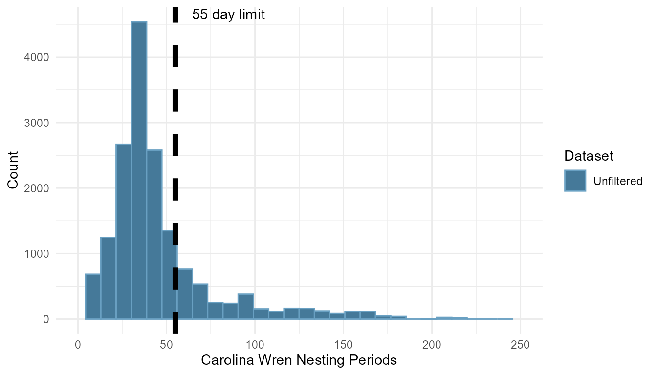
p2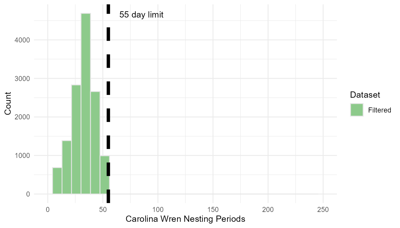
We can see in the unfiltered plot that there were more than a few nests with long nesting periods before filtering. After filtering out 448 attempts deemed “too long”, we are left with 2,539 attempts to continue an analysis with. Note that this function does not just trim the attempts by length. If you look closely you will see the distribution of nesting periods left of the cutoff has changed slightly (see the bar directly left of the dashed line has been reduced by several hundred attempts, and th other bars have increased slightly). This is due to removing days of nest checks post-fledging from the total nesting period.